Dear Organlearners,
Greetings to all of you.
I dedicate this contribution to fellow learner Alfred Rheeder. He does not
contribute as he would like to our LO-dialogue because their family
business keeps him very busy. The nature of the business affords profound
experiences in complexity. He calls upon me at least once a week with
provocative statements or daring questions on learning and complexity. The
meandering of his mind in the world of creativity and complexity astounds
me. About a month ago he asked me a question on entropic forces and fluxes
involving the "iron man competition". It set my mind working.
A couple of days ago Walter Derzko asked me some questions on learning
curves. It is then that I decided to write this contribution, giving
Alfred and Walter a context to explore their further questioning self.
I think that all of us have the following experience. When we have to
practice a definite skill, the first try takes the longest time and most
exertion. The second try takes a little bit less time and exertion. The
third try takes even less. However, the decrease between the second and
third try is not as much as between the first and second try. This pattern
repeats itself so that after some N tries the time and exertion each
stabilises at a minimum asymptotic value.
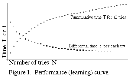
I have drawn in figure 1 the form of this pattern. Rick, will you please
in your kind manner archive this figure and supply us with its URL here:
http://www.learning-org.com/graphics/LO27588_curvetry.gif
Along the horizontal axis the number of tries N is depicted. Along the
vertical axis the differential time "t" taken to complete the task with
each try is depicted. Note the form of the curve which the data resulted
into. The form is called an exponential decrease. Also depicted along the
vertical axis (with another scale) is the cumulative time "T" for all
tries up to N tries. The form of this curve is called a logarithmic
increase.
Exponentially decreasing curves are abundant in the physical world. For
example, any radioactive substance disintegrates in an exponential manner.
When an electrical capacitor discharge through a resistor, its voltage
decreases exponentially. When any two compounds A and B are mixed so as to
react chemically, the amount of each decrease exponentially. When any
predator A enters a prisyine ecological niche to digest prey B, the prey
decrease exponentially.
Likewise curves with a logarithmic increase are abundant in the physical
world.
In the chemical sphere it became possible during the 20th
century to relate these exponential decreases to LEP (Law of
Entropy Production). What happens is that in any closed
system the entropy S increases. We symbolise it as
/_\S(sy) > O
where /_\ = "change", > = "is greater than" and
S(sy) = "entropy of system SY". The entropy S of the system
SY is maximised. This is the tail of the fish propelling it forward.
But the head of the fish guiding its course is the following. The
change /_\ of the entropy production /_\S(sy) is minimised, i.e.
/_\/_\S(sy) < 0
Consequently the system is attracted to an equilibrium where
the entropy S has a maximum value.
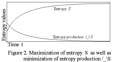
Such maximisation-minimisation curves are also known as a Lyapounov
functions. Study figure 2 (please Rick, supply the URL)
http://www.learning-org.com/graphics/LO27588_curventr.gif
I have drawn graphs of both the entropy S(sy) and the entropy production
/_\S(sy). Observe that the curve for the entropy S(sy) increases
logarithmically while the curve for the entropy production /_\S(sy)
decreases exponentially. When a logarithmic curve gets differentiated (the
action of the /_\) it results in an exponentially decreasing curve.
Conversely, when a curve with an exponential decrease gets integrated
(summed, accumulated), it results in a curve which a logarithmic increase.
Humankind has broken up Creation in so many topics and topics of topics
that few people are aware that such exponential and logarithmic patterns
occur in all walks of physical life. Even fewer are aware that these
patterns also occur in many walks of spiritual life. Furthermore, because
of confining LEP to physics, most humans who know something about LEP
think it is impossible for LEP to manifest itself in other walks of
physical life such as chemistry, geology, biochemistry, microbiology,
botany and zoology.
As for spiritual life, since the days of Descartes humankind had created
such a deep abyss between physical and spiritual life that no patterns are
acknowledged common to both. Where patterns appear to be the same, it is
ascribed to serendipity ("blind luck"). Hence when any person points to
correspondences between physical and spiritual patterns, such a person is
quickly ostracised because of not participating in "picking sides". How
dare this person not pay tribute to LEM (Law of Excluded Middle) -- select
either the one side or the other side, but neither both nor none? Stick to
the abyss! They claim that the physical and spiritual worlds are not one!
Exponentially decreasing patterns are also common to spiritual life.
Already several centuries ago artists like pianists (Beethoven and List),
painters, sculptors and poets knew that when they had to practise for
excellence in any particular skill, the time "t" it took them to complete
it each session, decreased like in figure 1. They also knew that they had
to have many skills. But when they had to practice one skill, they shut
out all thoughts on many other skills so as to focus all their mental
energy on this particular skill. Thus they managed to excel rapidly in
this skill so that they soon could shift to a new skill.
In 1926 Snoddy began to speak of learning curves and their "power law".
Arrow in 1962 and Alchian in 1963 introduced these learning curves into
economics. In 1981 Newell and Roosenbloom gave a review of empirical
learning curves as well as models for best fitting of these curves. Since
then it was open season for statisticians to propose best fitting models.
However, all these models lacked one thing -- a consistent theoretical
framework in which these models could be hooked. In the early nineties
budgeting with learning curves became standard in advanced accountancy.
In my opinion these curves are not as much learning curves as they are
performance curves. Learning involves the practising of many skills rather
than merely one, all to the level of excellence. Learning requires a
knowledge of when to leave the practising of one particular skill so as to
improve on it by practice other skills sustaining it. Learning also
requires the harmonising of many skills. Learning even requires the
awareness to still unknown skills needed to perfect a particular skill.
Learning is thus the complex matching of the performance curves of many
skills into one compelling symphony.
Unfortunately, as a result of the paradigm of the machine, especially
during the 20th century, workers were required to perform with excellence
in as few skills as soon as possible. Management then assembled these
workers in a production line to produce a commodity with the lowest costs
possible. Performance ("learning") curves became crucial to maximise
profits along the production line. The ability of humans to excel in many
skills was sold for making the biggest profit possible with mono-skills
assembled in a production line. Auditors were quick to point out in terms
of past performances which workers were failing to improve on their
performance curve. Assembly production became one big slavery driven by
the paradigm of the machine
Engineers tried their very best to make their machines as effective as
possible. Personnel managers followed suite trying to make workers as
effective as possible. But in such an assembly of mono-skills few, if
any, contemplated patterns intrinsic to both their systems, whether
physical or spiritual. One such a pattern is the most curious dichotomy of
properties into extensive or intensive properties. This is the very
outcome of LEP acting in the physical and spiritual worlds. When a system
is scaled up by an amount p, some properties increase by an amount p while
others stay exactly the same. Those properties which stay the same are
called intensive properties while those who scale up too are called
extensive properties.
For example, think of a dry cell with which we power our electronic
gadgets. By increasing its size with an amount p, its voltage remains the
same while its current output increases by p. Consequently voltage is an
intensive property while current is an extensive property. The electrical
energy which the cell has, is a product of its voltage and current.
Likewise can every form of energy may expressed as the product X.Y of two
factors, an extensive property X and its complementary intensive property
Y. (The dot "." between X and Y symbolises multiplication.)
When any form of energy X.Y changes, the X factor can change by /_\X or
the Y factor can change by /_\Y. The entropy production /_\S is not given
by (/_\X).Y or X./_\Y, but by /_\X./_\Y -- the full movie. It means that
both factors have to change. When a property has no /_\="change" fixed to
it, think of it as a static picture. But when a property has a /_\ fixed
to it, think of it as a dynamic movie. The /_\X is called an entropic flux
while the /_\Y is called an entropic force. When the system is scaled by
an amount p, the entropic fluxes (since they are derived from extensive
properties) get scaled by an amount p while the entropic forces (since
they are derived from intensive properties) stay the same.
Have you ever have thought of scaling mentally an organisation with which
you are involved? Should you do it, you will begin to discover which
properties are intensive (scaling independent) and which are extensive
(scaling dependent). As soon as a difference in an intensive property
arises it will act as an entropic force. For example, each section of the
organisation has its own manager. The organisation may scale (grow or
shrink), yet each section retains its one and only manager. It means that
the managers constitute an intensive property. Hence differences of
opinion between them on an issue will act as an entropic force.
No skill is possible without entropy production and the lowering of free
energy to sustain it. I am now going to indulge into mathematics which
will require some skill. any of you fellow learners might become
horrified. But there are a few who have that skill and we will need them
to make sure that what I am about to write is mathematically correct.
With each try practising that skill a certain amount /_\S(Z)
of entropy production is needed. The Z in /_\S(Z ) refer to
some or other common quantity like mass which we will
use to scale both the extensive properties X(Z) and the
intensive properties Y(Z). Let us now scale Z by a factor p
to the value p.Z (p dot Z) . Then we have for any extensive
property
X(p.Z) = p.X(Z)
and for any intensive property
Y(p.Z) = Y(Z)
Furthermore, we have for any entropic flux
/_\X(p.Z) = p./_\X(Z)
and for any entropic force
/_\Y(p.Z) = /_\Y(Z)
Consequently, since
/_\S(Z) = /_\X(Z)./_\Y(Z)
we have for the entropy production the scaling
/_\S(p.Z) = /_\X(p.Z)./_\Y(p.Z)
which becomes
/_\S(p.Z) = p./_\X(Z)./_\Y(Z)
so that we may conclude
/_\S(p.Z) = p./_\S(Z)
This result means that also the entropy production itself is
extensive. Compare the burning of a match with the burning
of a log. The log produces far more entropy than the match.
Since any skill s depends on entropy production /_\S which
itself is extensive, we expect the skill to be extensive too.
But fellow learners will remember that some two years ago
in the very long contribution
Efficiency and Emergence LO22426
< http://www.learning-org.com/99.08/0043.html >
I have explained carefully that we cannot have both efficiency
in a skill as well as emergences. Let us see what influence
does this have on skills.
Let us now write the skill s as a function s(N) of the number of tries N
it has been practised. Should all entropy production be focused on that
skill, then we may expect the skill s to be fully extensive. In terms of
the scaling factor p it means
s(p.N) = p.s(N)
However, if some of the entropy production is diverted
away to sustain some emergences, then the skill s will be
partially extensive. This means that
s(p.N) = q.s(N)
where
0 < q < p
so that the ratio q/p < 1. As q moves from p to 0 (zero),
the skill s becomes less extensive and thus more intensive.
It is this q < p which is responsible for performance curves.
There are also other reasons why all the entropy production
/_\S cannot be focussed on the skill s(N). For example,
some of the entropy production is needed to sustain other
skills on which the skill s(N), especially if the skill s(N) is
very complex. Furthermore, the person may try to increase
the entropy production by increasing the entropic forces
/_\Y far more than the entropic fluxes /_\X. In such a case
there will be a build up rather than an excretion of catabolic
(simpler) end products in the system, both physical and
spiritual. Lastly, chemistry warns us in terms of the order
and molecularity of any reaction how much a "one person"
skill differs from a "many person" skill. Thus we have to live
with the fact that
s(p.N) = q.s(N)
i.e., the skill s(N) is partially extensive.
I am going to show you fellow learners how to transform
the implicate function s(N) into an explicit form by making
use of the fact that it is partially extensive. Extend
s(p.N) = q.s(N)
into
s(p^r.N) = q^r.s(N)
where the p^r means p raised to the power r of it for all
r > 0. Let
x = 1 and s(1) = a.
Then
s(p^r.1) = q^r.s(1) = a.q^r
s(p^r) = a.q^r
Let
p^r = N
so that
r.ln p = ln N
where "ln" symbolises the natural logarithm. Now
r.ln q = (ln q/ln p).ln N
Let
(ln q/ln p) = 1 - b
in which we will call b the focussing power with
0 < b < 1
Then
ln q^r = ln N^(1 - b)
so that
q^r = N^(1 - b)
Using this and
p^r = N
in
s(p^r) = a.q^r
gives
s(N) = a.N^(1 - b)
Thus we have succeeded in making the skill s(N) explicit
in terms of the number of tries N and two constants a and b.
Please refer again to figure 1. One of the most easiest ways
to measure the improved performance of a skill s(N) is to
do it in terms of the total time T which it takes to complete
N tries in exercising that skill. We measure the time t(i) for
each try i and then add them up one after another. In other
words, let the cumulative time T(N) be defined by
T(N) = SUM[i: 1 to N][t(i)]
We will now express the skill s(N) by T(N) as its
measurement. The formula
T(N) = a.N^(1 - b), N=1, 2, 3, ....
represents "exactly" the data for the cumulative time T. It is
the curve which increases logarithmically.
Should we define
T(N)/N = T/N
as the average cumulative time, the formula
T/N = a.N^(-b)
will represent closely the data for differential time t per
each try. It is the curve which decreases exponentially.
I wrote "exactly" because the formula
T(N) = a.N^(1 - b)
will not fit the data exactly. Firstly, we have to keep in
mind fluctuations as a result of minor interactions with the
environment. Secondly, we have to keep in mind that
entropy is produced by more than one entropic force-flux
pair. Thirdly, as we soon will see, the creativity of the
performer will have a great influence on the performance
curve. So if we want a better statistical fit, we will have to
extend the formula to its "bi-power" form
T(N) = a.N^(1 - b) + c.N^(1 - d)
where we have to determine four constants a, b, c and d.
It will usually give a very good fit. If not, the "tri-power"
form
T(N) = a.N^(1 - b) + c.N^(1 - d) + e.N^(1 - f)
will have to be used.
A concept often encountered in performance (learning)
curves is the "Doubling Ratio" DR. It is the ratio between
the cumulative time T(N) for the N-th try to that for the
2N-th try. This is given by
DR = T(N)/T(2N)
= a.[N^(1 - b)]/[a.(2N)^(1 - b)]
= 2^(b - 1)
Since
0 < b < 1
the doubling ratio DR has the limiting values
0.5 > DR > 1.0
because 2^-1 = 0.5 (50%) and 2^0 = 1.0 (100%)
Let us see how focussing power b influences the cumulative performance
curve. Observe figure 3. (Please Rick, supply the URL)
http://www.learning-org.com/graphics/LO27588_curveper.gif
The scale of the bottom curve has been increased while the scale of the
top curve has been decreased to fit them all nicely into one figure.
Assume the focus b = 0.9, i.e very close to its maximum value 1.0. Then
the DR = 0.93. We can also say that the performance curve is 93% flat. It
is the bottom curve on figure 3. Assume b = 0.1, i.e very close to its
minimum value 0. The DR = 0.53. We say that the performance curve is 53%
flat. It is the top curve on figure 3. The middle curve is 71% flat with
b = 0.5
There is a tendency to misuse the performance curves by saying that
somebody with focus b close to 0 and DR close to 50% flat is clumsy or
foolish while somebody with b close to 1 and DR close to 100% flat is
agile or intelligent. This has to be deplored. It is rather a case of how
the performer match up to complexity. One and the same person will perform
a simple task with b = 0.9 and DR = 93%, but a complex task with b = 0.1
and DR = 53%. Furthermore, as the learner is exposed to a more complex
environment and learn how to live with it, both the focussing power b and
the doubling ratio DR will increase. Performance curves will become less
steep.
People often think that by practising a skill many times will
improve its performance. It is true because according to
the formula
T(N) = a.N^(1 - b)
that person will indeed move along the logarithmic curve
by increasing N. See figure 3. However, the exceptional
performer also does something else, namely to decrease
the initial performance time T(1)=a and to increase the
focussing power b. In other words, the exceptional
performer tries to transform him/herself from a curve like
the top one (b = 0.1 and DR = 93%) to a curve like the
bottom one (b = 0.9 and DR = 53%). It is as if the
exceptional performer bends the curve more horizontal
(by increasing b) and also pushes it downwards (by
decreasing T(1)=a).
The initial performance time T(1)=a may be decreased
by proceeding from one to many skills -- a
"one-to-many-mapping" of skills. Every skill is related by
a network to many other skills. The more the number of
such related skills which had been practised (and obviously
the number of practices in each related skill to increase its
performance), the more they will help to decrease the initial
performance time T(1)=a of a new skill to be practised.
Thus it is a good strategy to practice as many skills as
possible. A performer may not yet know which of them
will aid the practising of the new skill, but some of them
will certainly do so.
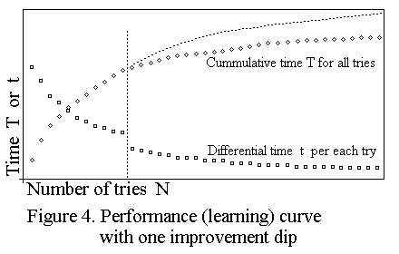
This decreasing of T(1)=a need not necessarily be accomplished in advance.
The performer may suddenly realise during the N-th practice of a certain
skill that another sustaining skill had not been practised. Hence the
performer ought to practise that other skill before returning to the skill
being practised. This means that at some stage in the performance curve of
any particular skill, the performer will suddenly stop improvising or will
even seem to be deteriorating in that skill. It is because the person's
entropy production /_\S is needed to develop that other skill. But when
the performer return to the skill being practised, the cumulative
performance curve T will dip into a flatter progression. See figure 4.
(Please Rick, supply the URL)
http://www.learning-org.com/graphics/LO27588_curvedip.gif
On the other hand the, differential performance curve t will show a clear
step downwards depicting shorter times t to repeat the skill.
The effect of decreasing T(1) = a some where along the sequence of
practices at say the N-th try, is like cutting out the (N+1)-th, (N+2)-th,
..., (N+n)-th try and then adding the remainder (N+n+1)-th, (N+n+2)-th,
... to the N-th try. Thus there is actually no waste of free energy and
entropy production by shifting to another sustaining skill, improve on it
by practising it for a number of tries and then returning to the former
skill to improve further on it by practising from the seemingly (N+n)-th
try.
The focussing power b is also often known as performance concentration --
the "mental adrenalin pumped into the performance". It is here where the
7Es (seven essentialities of creativity) liveness, sureness, wholeness,
fruitfulness, spareness, otherness and openness come into play. These 7Es
express the form of the performance in a 7th-fold manner. The more the
performer is aware of each of them and incorporate them into the
performance, the greater is the focussing power b. It means that
creativity optimises the focussing power b.
Creative performers will carefully contemplate the complexity of the skill
to be practised even before the first practice T(1)=a. This will let b
increase most. Then, after the first practice and before the second
practice T(2), they will again evaluate the first practice so as to
improve deliberately on the second practice. This will let b increase
slightly more. By doing the same after the second practise, b will
increase even more, but less than after the first practise. Creative
performers will do the same after each subsequent practise. In other
words, in any complex skill they will let b itself improve in a
logarithmic manner from close to b = 0 to close to b = 1! They begin with
practising the skill like the top curve of figure 3, but soon ends with
practising it like the bottom curve of figure 3. This consecutive
contemplation is sometimes also called AAR (After Action Review).
It is not possible to get a good fit (for example, using a
P-test) for the performance of a creative performer with the
mono-power formula
T(N) = a.N^(1 - b)
To get a good fit, at least the "bi-power" formula
T(N) = a.N^(1 - b) + c.N^(1 - d)
will have to be used. Thus it is actually possible to express
the performer's creativity during the performance of by the
ratio of fitting (say P values of the P-test) of the "bi-power"
formula
T(N) = a.N^(1 - b) + c.N^(1 - d)
to the "mono-power" formula
T(N) = a.N^(1 - b)
The greater this ratio, the more creative the performance
curve of the skill.
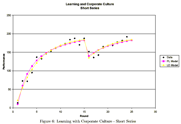
Should you fellow learners want to look as some graphs
involving empirical data, have a look at
< http://www.cebiz.org/cds/macleod.pdf >
from p37 to p44. As for the previous pages, save yourself
from a much worse mathematical nightmare ;-) If you do
not have Acrobat reader installed, you might take a look
at one of the figures (Please Rick, supply the URL)
http://www.learning-org.com/graphics/LO27588_curvefi6.gif
Dear fellow learners, I want to thank Alfred Rheeder for the many
provocative statements or daring questions which he fired at me the past
month on improving performances. It helped me a lot to form this
contribution in my mind. His diligent attempts to coordinate his answers
with what he already knows of entropy production, had been a source of
inspiration to me.
Alfred, I think you will agree with me that the curves
depicted in figure 1 are not so much learning curves as they
are performance curves. The shape of a
T(N) = a.N^(1 - b)
curve is determined by how much the entropy production
is utilised. This is given by the partial extensive
s(p.N) = q.s(N)
where
0 < q < p
We have defined the focus power b specifically as
b = (ln q/ln p)
When the skill s is fully extensive like the entropy production
/_\S(p.Z) = p./_\S(Z)
i.e., q = p, then the focus power b = 1.
To learn is not to follow the shape of the curve
T(N) = a.N^(1 - b)
but to change its shape by decreasing a = T(1) and by
increasing the focus power b. It means that to learn is to
press the performance curve lower (by decreasing a) and
to bent it more horizontally (by increasing b). In terms of
figure 3 it means to move from the top curve to the bottom
curve using all possible means.
Alfred, your task as a coach (among the many tasks which you have) is not
to understand this contribution. I think your performance curve is such
that you will understand it after having worked through it a few times.
Your task as a coach will be to make sense to your subjects who do not
have the low a = T(1) and high b which you have. For them only one thing
exists -- to go rotely (mechanically) through their fixed performance
curve
T(N) = a.N^(1 - b)
so many times N that they finally drop dead or injure
themselves permanently.
With care and best wishes
--At de Lange <amdelange@gold.up.ac.za> Snailmail: A M de Lange Gold Fields Computer Centre Faculty of Science - University of Pretoria Pretoria 0001 - Rep of South Africa
Learning-org -- Hosted by Rick Karash <Richard@Karash.com> Public Dialog on Learning Organizations -- <http://www.learning-org.com>
"Learning-org" and the format of our message identifiers (LO1234, etc.) are trademarks of Richard Karash.